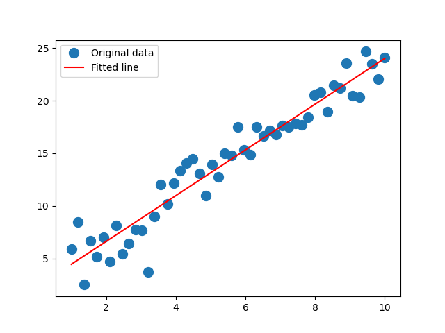
General Linear Least Squares Fitting

You might have heard of linear regression for fitting a straight line to data, such as in the picture below. But did you know that you can fit much more complicated functions to data, and the procedure is almost as simple? You may be surprised to learn that “linear” covers a lot more than straight lines. This article is looking at the general “linear least squares” problem. So why is it called “linear” then? We’ll get to that.

Linear least-squares regression fit (red line) to noisy data (blue dots)

As we’ll see below, the math becomes a lot simpler but also more generally useful when we introduce Linear Algebra and matrices. But first we consider the common case of fitting a straight line, without the use of matrices.

That is, we do a straight line fit the hard way.

Linear Regression (straight-line fitting, non-matrix version)

Often we have data that is noisy as with the blue dots in the figure, and we are interested in the trend line. We believe that the “true” y data follows a straight-line relationship with respect to x,

$y = m x + b$

but has been corrupted by noise, so instead the observed y values are a little above or below the true y data.

$y_i = m x_i + b + \varepsilon_i$

where the term $\varepsilon_i$ refers to a random error that has been added to the i-th data point.

Statistics Note: (If statistical language triggers you, skip this paragraph.) For the statistical analysis of this procedure, you need to know that most commonly the errors are assumed to come from a normal distribution with mean = 0, and they are independent. Also, they all have the same standard deviation. If you drew the error bars, they would all be the same size. We’re not doing a statistical analysis, but you can assume we keep those assumptions because the “best” fit is different if they don’t hold.

Note that the equation above with the error term is for the purpose of the analysis. We don’t have access to the error value and the “true y”. All we have is a measured $y_i$ for each $x_i$ . This is our blue dot. We then have a predicted or estimated y value for that $x_i$ , and we indicate that with a hat: $\hat{y}_i = \hat{m} x_i + \hat{b}$ . The hats on m and b indicate that they too are estimated values, our best guess at the true values.

Statistics Note: In statistics terms, $\hat{m}$ and $\hat{b}$ are estimators of the true values $m$ and $b$ . The “best fit” procedure is the one that gives good estimators, which usually to a statistician means unbiased (it’s the right value on average) and minimum variance (most guesses are closer for this procedure than others). This is what I meant when I said the “best” fit is different for a different error model. Again, I’m not going to actually do a statistical analysis here but I assure you there is plenty of material out there if you want to find one.

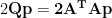
So what is the procedure? For any particular guess at the parameters $\hat{m}$ and $\hat{b}$ , we can calculate the residuals on each data point, the difference $(y_i - \hat{y}_i)$ between measured and predicted y value for each point.

Some will be positive, some negative, so what we do is square them, and add them up. That gives us this quantity (assuming we have $n$ data points), the total squared error:

$\displaystyle E(\hat{m}, \hat{p}) = \sum_{i=1}^n \left (y_i - \hat{y}_i \right )^2$

The $x_i, y_i$ are fixed in this expression. Do not think of them as variables. Instead, think of $\hat{m}$ and $\hat{b}$ as the variables. If we change those parameters, we get a different trend line, different residuals, and a different calculated value of E. The goal in least-squares fitting is to find the parameters which give us the lowest possible value of the total squared error E.

In other words, we are going to minimize the function E with respect to the variables $\bf\hat{m}$ and $\bf\hat{b}$ .

So that means we’re going to take the derivatives with respect to those variables and set them equal to 0.

First we expand E in terms of the parameters. For simplicity we’ll just write $\sum_i$

$\displaystyle E = \sum_i \left (y_i - \hat{y}_i \right )^2 \\ = \sum_i \left( y_i - \hat{m} x_i - \hat{b} \right )^2 \\ = \sum_i \left (y_i^2 + \hat{m}^2 x_i^2 + \hat{b}^2 - 2\hat{m}y_i x_i - 2\hat{b} y_i + 2\hat{m} \hat{b} x_i \right ) \\ = \sum_i y_i^2 + \hat{m}^2 \sum_i x_i^2 + n \hat{b}^2 - 2\hat{m} \sum_i y_i x_i - 2\hat{b} \sum_i y_i + 2\hat{m} \hat{b} \sum_i x_i$

The n in the third term comes from the fact that we are adding a $\hat{b}^2$ term for each i, a total of n such terms. Now we take the derivatives.

$\displaystyle \frac{\partial E}{\partial \hat{m}} = 2\hat{m} \sum_i x_i^2 - 2\sum_i y_i x_i + 2\hat{b} \sum_i x_i = 0\\ \frac{\partial E}{\partial \hat{b}} = 2n\hat{b} - 2\sum_i y_i + 2\hat{m}\sum_i x_i = 0$

(Remember, the derivatives are with respect to the hatted parameters. The summations over data values are constants.) The second equation can be rearranged to

$\displaystyle \hat{b} = \frac{\left (\sum_i y_i - \hat{m} \sum_i x_i \right )}{n}$

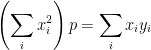
This can be used to find the value of $\hat{b}$ once $\hat{m}$ is known. Substituting that into the first equation (and dividing out the 2)

$\displaystyle \hat{m} \sum_i x_i^2 - \sum_i y_i x_i + \frac {\left ( \sum_i y_i - \hat{m} \sum_i x_i \right )} {n} \sum_i x_i = 0 \\ \hat{m} \left [ \sum_i x_i^2 - \frac {\left (\sum_i x_i \right )^2}{n} \right ] - \sum_i y_i x_i + \frac {\left ( \sum_i y_i \right )\left ( \sum_i x_i \right )}{n} = 0 \\ \hat{m} \left [ n \sum_i x_i^2 - \left (\sum_i x_i \right )^2 \right ] - n\sum_i y_i x_i + \left ( \sum_i y_i \right )\left ( \sum_i x_i \right ) = 0$

Giving us the standard linear regression equations:

$\displaystyle \hat{m} = \frac {\left [ n\sum_i y_i x_i - \left ( \sum_i y_i \right )\left ( \sum_i x_i \right ) \right ]} {\left [ n \sum_i x_i^2 - \left (\sum_i x_i \right )^2 \right ]} \\[6pt] \hat{b} = \frac{\left (\sum_i y_i - \hat{m} \sum_i x_i \right )}{n}$

Whew! That was a heck of a lot of algebra!

Now watch how easy this becomes when we apply linear algebra.

Linear Regression (straight-line fitting, matrix version)

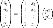
We define a column vector $\bf{x} = (x_1, x_2, \hdots, x_n)^T$ of our x values and similarly $\bf{y} = (y_1, y_2, \hdots, y_n)^T$ of our observed y values. Our fitted y values from the model are $\bf{\hat y} = (\hat{y}_1, \hat{y}_2, \hdots, \hat{y}_n)^T$ .

Anticipating the more general fitting problem, we will give our unknown parameters the names $p_0$ (for the constant term) and $p_1$ (for the slope, the coefficient of $x$ ). Then

$\displaystyle \bf{\hat{y}} = p_0 + p_1 \bf{x}$

and the residuals can be expressed as $(\bf{y} - \bf{\hat y})$ .

Let’s define a parameter vector $\displaystyle \bf{p} = \begin{pmatrix} p0 \\ p1 \end{pmatrix}$ . Then we can write a matrix equation for the predicted $\hat{y}$ values:

$\displaystyle \begin{pmatrix}\hat{y}_1 \\ \hat{y}_2 \\ \vdots \\ \hat{y}_n \end{pmatrix} = \begin{pmatrix}1 & x_1 \\ 1 & x_2 \\ \vdots & \vdots \\ 1 & x_n \end{pmatrix} \begin{pmatrix}p0 \\ p1 \end{pmatrix}$

or $\bf{\hat{y}} = \bf{Ap}$ where A is the n x 2 matrix whose first column is the number 1 and second column contains the x values. So the residual vector is $(\bf{y} - \bf{Ap})$ .

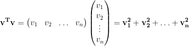
Recall that for any vector $\bf{v} = (v_1, v_2, \hdots, v_n)^T$ , the magnitude squared or the sum of the squared components is

$\displaystyle \bf{v^Tv} = \begin{pmatrix} v_1 & v_2 & \hdots & v_n \end{pmatrix} \begin{pmatrix} v_1 \\ v_2 \\ \vdots \\ v_n \end{pmatrix} = v_1^2 + v_2^2 + \hdots + v_n^2$

So the total squared residual E can be written as

$\displaystyle E = (\bf{y} - \bf{Ap})^T (\bf{y} - \bf{Ap})$

Expanding a product like this in linear algebra isn’t that different from ordinary algebra, using the Distributive Law (you may have learned the technique called FOIL or First, Outer, Inner, Last). The difference in matrix expressions is that you should keep products in the order they occurred because AB is not in general the same as BA.

We also need the property that the transpose of a product reverses the order of multiplication, i.e., that 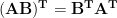$\bf{(AB)^T} = \bf{B^TA^T}$ so $\bf{(Ap)^T} = \bf{p^TA^T}$ .

$\displaystyle E = (\bf{y}^T - \bf{p^TA^T}) (\bf{y} - \bf{Ap}) \\[6pt] = \bf{y^Ty} - \bf{y^TAp} - \bf{p^TA^Ty} + \bf{p^TA^TAp}$

Our vectors such as $\bf{y}$ and $\bf{Ap}$ are all n x 1 column vectors, and their transposes are 1 x n row vectors. So every term here is a 1 x 1 scalar, a simple number, since of course E is a simple number representing the total squared error.

The middle two terms are transposes of each other, but since they are scalars, the transposes are equal, representing the same number. So we can combine them.

$\displaystyle E = \bf{y^Ty} - 2\bf{y^TAp} + \bf{p^TA^TAp} = \bf{y^Ty} - 2\bf{(A^Ty)^Tp} + \bf{p^T(A^TA)p}$

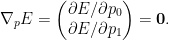
We want to minimize this with respect to $\bf{p}$ . That is, we want to find the value of $\bf{p}$ such that $\nabla_p E = \begin{pmatrix} \partial E / \partial p_0 \\ \partial E / \partial p_1 \end{pmatrix} = \bf{0}.$

The first term is constant with respect to $\bf{p}$ , so its gradient is 0. The second term has the form $\bf{a^Tp}$ with $\bf{a} = 2\bf{A^Ty}$ and its gradient is equal to $\bf{a} = 2\bf{A^Ty}$ . The third term has the form $\bf{p^TQp}$ with $\bf{Q} = \bf{A^TA}$ and its gradient is equal to $2\bf{Qp} = 2\bf{A^TAp}$ .

(For proofs of those gradients, see this post)

Thus the least squares solution for $\bf{p}$ satisfies

$\displaystyle -2\bf{A^Ty} + 2\bf{(A^TA)p} = 0 \\[8 pt] \bf{(A^TA)p} = \bf{A^Ty}$

This is a linear system of equations for $\bf{p}$ of the form $\bf{Bp} = \bf{b}$ . $\bf{A^T}$ is 2 x n and $\bf{A}$ is n x 2, so $\bf{B} = \bf{A^TA}$ is 2 x 2.

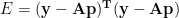
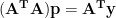
This is a general result. We started by asking what vector $\bf{p}$ minimizes $E = (\bf{y} - \bf{Ap})^T (\bf{y} - \bf{Ap})$ . If a problem can be put in this form, the solution is the vector which solves the linear system $\bf{(A^TA)p} = \bf{A^Ty}$ .

We often in linear algebra run into overdetermined systems (more equations than unknowns) of the form $\bf{Ax} = \bf{b}$ with no exact solution. In these cases the best approximate solution, the one that minimizes the magnitude of the difference between $\bf{Ax}$ and $\bf{b}$ . The linear regression problem with n rows and 2 columns is just one example.

As we’ll see below, a much wider class of problems than linear regression fits this framework, and all those problems can be solved the same way. Because the equations are a linear system in terms of the unknown parameters, all such problems are considered linear least-squares.

The system $\bf{(A^TA)p} = \bf{A^Ty}$ is a system of linear equations. Software to solve linear systems is available in many computer languages and mathematics libraries. Python has one called numpy.linalg.solve, and Matlab has the backslash operator (\). So one approach is to build $\bf{(A^TA)}$ , build $\bf{A^Ty}$ and then give them to a linear system solver to find the unique exact solution of this system, which will be the best least-squares to the original overdetermined system.

But both those languages also have the built-in capability to find the least-squares solution of an overdetermined system. Python has numpy.linalg.lstsq, and Matlab’s backslash operator will calculate the least-squares solution if the system is overdetermined. So in fact all you have to do is construct $\bf{A}$ and $\bf{y}$ .

To summarize, the way to do linear regression with linear algebra is:

Create the 2-column matrix $\bf{A}$ whose first column is all 1’s and second column is the ${x_i}$ values.
Create a column vector $\bf{y}$ of the ${y_i}$ values.
If your computer environment has a least-squares system solver, use it to find the least squares solution $\bf{p}$ of $\bf{Ap} = \bf{y}$ .
Otherwise, compute $\bf{A^TA}$ and $\bf{A^Ty}$ and use a linear system solver to find the solution $\bf{p}$ of the system $\bf{(A^TA)p} = \bf{A^Ty}$
The elements of $\bf{p}$ are the least-squares values of intercept and slope, in that order.

Here is the Python code that performed the fit and plotted the results that appear at the top of this page. This code is modeled from the example code at https://numpy.org/doc/stable/reference/generated/numpy.linalg.lstsq.html.

A = np.vstack([np.ones(len(x)),x]).T
p = np.linalg.lstsq(A, y, rcond=None)[0]
plt.plot(x, y, 'o', label='Original data', markersize=10)
plt.plot(x, p[1]*x + p[0], 'r', label='Fitted line')
plt.legend()
plt.show()

Notice that the actual regression only took two lines here. The other four lines are to generate the plot.

General Linear Least Squares

All of the method above is based on the equation $\hat\bf{y} = \bf{Ap}$ . If the model for $\hat\bf{y}$ can be written in that form, then the total squared error has the form we saw above and the optimum least-squares solution has exactly the same form. All we need is to properly define the matrix $\bf{A}$ .

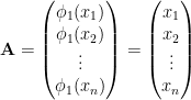
We can do this as long as our model has the form

$\hat\bf{y} = p_1 \phi_1(x) + p_2 \phi_2(x) + \cdots + p_r \phi_r(x)$

i.e., a sum of $r$ functions multiplied by unknown coefficients ${p_k}$ , which we will optimize in the least-squares sense.

This has the matrix representation $\hat\bf{y} = \bf{Ap}$ if $\bf{A}$ is the matrix whose $(i, j)$ -th elements is $\phi_j(x_i)$ . The $j$ -th column contains the value of the function $\phi_j$ evaluated at each of the x values.

For linear regression, we have $\phi_1(x) = 1$ and $\phi_2(x) = x$ . This is easily extended to polynomials of any degree by adding columns for $\phi_3(x) = x^2$ , $\phi_4(x) = x^3$ , etc.

But it is much more general than that, since the $\phi_k$ can be any function at all. We’ll see some examples in the next section. The general method is virtually the same as linear regression, but generalizing the first step.

Create the r-column matrix $\bf{A}$ where the $j$ -th colum consists of $\phi_j(x_i)$ evaluated at each $x_i$ .
Create a column vector $\bf{y}$ of the ${y_i}$ values.
If your computer environment has a least-squares system solver, use it to find the least squares solution $\bf{p}$ of $\bf{Ap} = \bf{y}$ .
Otherwise, compute $\bf{A^TA}$ and $\bf{A^Ty}$ and use a linear system solver to find the solution $\bf{p}$ of the system $\bf{(A^TA)p} = \bf{A^Ty}$
The elements of $\bf{p}$ are the least-squares values of intercept and slope, in that order.

Examples of the general method

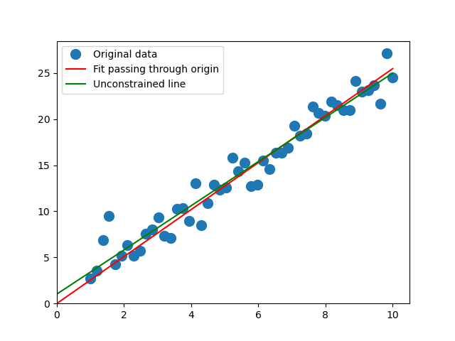
Line constrained to go through the origin

Sometimes we want a line where the y-intercept is forced to be 0. In this case, there’s only one parameter, the slope. It’s a little bit of overkill to use a computer linear algebra system to solve this problem, but we can still take advantage of the equations to immediately write down the solution.

Since we only have one function $\phi_1(x) = x$ , our matrix $\bf{A}$ is now just the column of $x$ values.

$\displaystyle \bf{A} = \begin{pmatrix} \phi_1(x_1) \\ \phi_1(x_2) \\ \vdots \\ \phi_1(x_n) \end{pmatrix} = \begin{pmatrix} x_1 \\ x_2 \\ \vdots \\ x_n \end{pmatrix}$

Then $\bf{A^TA}$ is $\sum_{i} x_i^2$ and $\bf{A^Ty}$ is $\sum_{i} x_i y_i$ . The “system” to solve is

$\displaystyle \left (\sum_{i} x_i^2 \right ) p = \sum_{i} x_i y_i$

$\displaystyle p = \frac {\sum_{i} x_i y_i}{\sum_{i} x_i^2}$

is the optimal slope. The figure below shows a fit using this model, compared to an ordinary linear regression with a nonzero y-intercept.

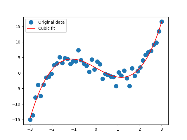
Linear regression to a set of data with y-intercept constrained to be 0 (red line) and unconstrained (green line)

Cubic polynomial

The model here is $\hat{y} = p_1 + p_2 x + p_3 x^2 + p_4 x^3$ so our functions are $\phi_1 = 1, \phi_2 = x, \phi_3 = x^2 and \phi_4 = x^3$ . The $\bf{A}$ matrix contains those powers of x as its columns.

Again we use Python’s numpy.linalg.lstsq() to calculate the least-squares solution to $\bf{Ap} = \bf{y}$

A = np.vstack([np.ones(len(x)),x,x*x,x**3]).T
p = np.linalg.lstsq(A, y, rcond=None)[0]

The result is shown in the figure below.

Linear least-squares fit of a cubic polynomial

Sinusoid

If we are trying to fit a model of the form 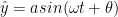$\hat{y} = a sin(\omega t + \theta)$ , we cannot use the linear least squares procedure to find $\omega$ because it does not appear as a term of the form $\omega \phi(x)$ . The model is not linear in the parameter $\omega$

However, despite the fact that the phase shift $\theta$ is also a nonlinear parameter, we can fit a phase-shifted sinusoid to data, because a phase shifted sinusoid can be represented as a sum of an unshifted sine and cosine.

$\displaystyle sin(a + b) = sin(a) cos(b) + cos(a) sin(b) \\ a sin(\omega t + \theta) = [a cos(\theta)] sin(\omega t) + [a sin(\theta)] cos(\omega t)$

So we will use a model with $\phi_1(t) = cos(\omega t)$ and $\phi_2(t) = sin(\omega t)$ , and $\omega$ is either known or estimated by other means.

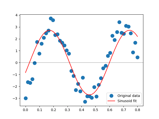
The result is shown below. The original data had a frequency of 2 Hz, so $\omega = 4\pi = 12.57$ . In practice you could have some procedure to estimate the frequency so might not obtain the correct value. To simulate that, we used a value of 11 in this fit.

Linear least squares fit of a phase-shifted sinusoid, represented as a sum of an unshifted sine and cosine term. Angular frequency “estimate” of $\omega = 11$ was used (actual value 12.57)

Linear least squares fit of a phase-shifted sinusoid, represented as a sum of an unshifted sine and cosine term. Angular frequency “estimate” of $\omega = 11$ was used (actual value 12.57)

Terra Physicae Mathematicaeque (Terra-Phy)